Polynomials
MATLAB contains a variety of functions that help with polynomials. This includes evaluating polynomials, finding their roots, and doing some basic arithmetic. Using these functions will accelerate your work and make your scripts easier to understand.
The MATLAB Help Center includes guides for these functions on their Polynomials page.
\[f(x) = \sum_{i=1}^n p_i x^{n-i} = p_1 x^{n-1} + p_2 x^{n-2} + \dots\]Creating Polynomials
The equation above is the general form of a polynomial. It is a series of powers of $x$, each with their own coefficient. For example, the polynomial $y = 3 x^2 - 10 x + 1$ has coefficients $[3, -10, 1]$. When extracting the coefficients into a list like this, it is import to first put the terms in order so the power on $x$ is decreasing. If you have a polynomial with missing powers, like $y = 3 x^4 - 10 x + 1$, you need to put zeros in places where the powers are missing.
\[3 x^4 - 10 x + 1 \Rightarrow 3 x^4 + 0 x^3 + 0 x^2 - 10x + 1 \Rightarrow [3, 0, 0, -10, 1]\]Creating the above polynomial in MATLAB is a matter of defining an array that contains the coefficients.
% 3x^4 - 10x + 1
p = [3, 0, 0, -10, 1];
Practically, MATLAB does not treat this array differently from others. What matters is how we use this array in polynomial-specific functions.
Evaluating Polynomials
To evaluate the value of a polynomial at a value of $x$, use the polyval function.
The syntax is y = polyval(p, x), where p is the array of coefficients and x is the input.
Example: Pumpkin Cannon
Question
At the Punkin Chunkin annual event, a compressed air cannon accelerates a pumpkin to a speed of 100 mph. Assuming the barrel is angled 45 degrees relative to the ground and the pumpkin has an altitude of 15 ft when it leaves the cannon, how high (in feet) does the pumpkin get 2 seconds after leaving the cannon?
%% Units
% English
U.S = 1;
U.MIN = 60*U.S;
U.HR = 60*U.MIN;

U.FT = 1;
U.MILE = 5280*U.FT;

U.RAD = 1;
U.DEG = pi*U.RAD/180;

%% Givens
speed = 100*U.MILE/U.HR;
theta = 45*U.DEG;
h_0 = 15*U.FT;
dt = 2*U.S;

%% Constants
g = 32.2*U.FT/U.S^2;
Solution
You can find the height of the pumpkin at 2 seconds using the formula:
\[h(t) = -\frac{1}{2} g t^2 + v_0 t + h_0\]The speed in this equation is only the vertical component, so we use the barrel angle to determine how fast the pumpkin is traveling in the vertical direction. These are combined in a script that looks like:
%% Units
% English
U.S = 1;
U.MIN = 60*U.S;
U.HR = 60*U.MIN;

U.FT = 1;
U.MILE = 5280*U.FT;

U.RAD = 1;
U.DEG = pi*U.RAD/180;

%% Givens
speed = 100*U.MILE/U.HR;
theta = 45*U.DEG;
h_0 = 15*U.FT;
dt = 2*U.S;

%% Constants
g = 32.2*U.FT/U.S^2;

%% Calculation

% Vertical speed
v_vert = speed * sin(theta);

% Height vs time, without air resistance
% h(t) = -1/2*g*t^2 + v_0*t + h_0
p = [-1/2*g, v_vert, h_0];

% Height at dt
h = polyval(p, dt);

%% Answer
disp(['Height at ' num2str(dt/U.S) ' s: ' num2str(h/U.FT) ' ft'])
Which produces this result:
Height at 2 s: 158.018 ft
MATLAB can also accept arrays for the variable x, in addition to single values.
In the example above, dt could be a range of times and we could later
plot the trajectory like plot(dt, polyval(p, dt)).
If we do not know the time of flight initially, we could set dt to be a range then mask values where the height is negative.
For example:
poly_pumpkin_cannon  % the script in the example

%% Evaluate entire trajectory
dt = (0:0.01:100)*U.S;
h = polyval(p, dt);

%% Plot trajectory above ground
mask = h >= 0;
plot(dt(mask)/U.S, h(mask)/U.FT, ...
     'Color', '#FF7518', ... % pumpkin color
     'LineWidth', 2);
ylim([0 inf])  % force lower bound to be y=0
grid('on')
xlabel('Time [s]')
ylabel('Height [ft]')
title('Pumpkin Height vs Time')
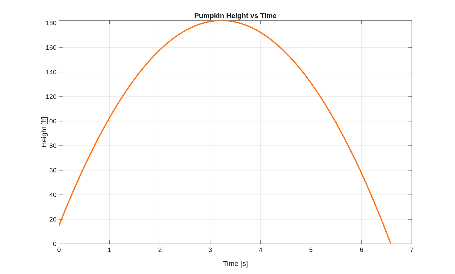
Here, we reasonably assume it will take no more than 100 seconds for the pumpkin to reach the ground.
The polyval function will evaluate the polynomial p as if there was no ground and the pumpkin kept falling.
Masking on heights above ground level avoids plotting those values.
The MATLAB Help Center has documentation on polyval.
Roots of Polynomials
Another common operation on polynomials is determining their roots.
These are values of x where the polynomial evaluates to zero.
In the pumpkin example, the roots of that polynomial are the times when the pumpkin has zero height.
The MATLAB command is roots and the syntax is simply r = roots(p).
Continuing with the pumpkin example:
poly_pumpkin_cannon  % the script in the example

%% Evaluate roots
r = roots(p)

%% Find time of flight
tf = max(r);
disp(['Time of flight: ' num2str(tf/U.S) ' s'])
r =

    6.5831
   -0.1415

Time of flight: 6.5831 s
A polynomial of degree $n$, which is the largest power of $x$, always has $n$ roots.
Sometimes these roots are complex, sometimes they are repeated,
but there are always the same number of roots as the order of the polynomial.
In fact, the roots of a polynomial can be used to calculate the equivelant polynomial coefficients.
This function is called poly and it is like the inverse of roots.
Its syntax is p = poly(r).
This is useful in situations where you have a list of desired root locations and
need to find the equivalent polynomial for other analyses.
The MATLAB Help Center has documentation on roots and poly.
Polynomial Arithmetic
Sometimes we need to perform arithmetic operations on two polynomials like add, subtract, multiply, and divide.
To add two polynomials together, first we need to make sure their arrays are the same length.
We do this using the zeros function, which will pad an array with leading 0s.
For example:
% Adding polynomials
%
%     3x^3 + 1x^2 - 8x +  2
% +                 6x - 10
% --------------------------
%     3x^3 + 1x^2 - 2x -  8

p1 = [3 1 -8 2];
p2 = [6 -10];

padded_p2 = [zeros(1,2) p2]
p3 = p1 + padded_p2
padded_p2 =

     0     0     6   -10


p3 =

     3     1    -2    -8
Subtracting two arrays follows the same process as adding, with - instead of +.
To multiply two polynomials together, use the conv function (short for convolution).
Its syntax is conv(p1, p2) and it will do all of the first-outside-inside-last for you,
regardless of how long the polynomials are.
You do not need to pad the shorter polynomial when using conv.
As an example:
% Multiplying polynomials
%
%     3x^3 + 1x^2 - 8x +  2
% x                 6x - 10
% --------------------------
%    18x^4 + ... - 20

p1 = [3 1 -8 2];
p2 = [6 -10];

p3 = conv(p1, p2)
p3 =

    18   -24   -58    92   -20
The most challenging of the four operations mentioned is dividing polynomials.
This is performed using deconv, which has syntax [x, r] = deconv(p1, p2).
The numerator is p1 and the denominator is p2.
The output x is the “whole number” quotient while r is the remainder.
Mathematically, you could recover p1 by doing p1 = conv(x, p2) + r.
As an example:
% Dividing polynomials
%
%     3x^3 + 1x^2 - 8x +  2
% ÷                 6x - 10
% --------------------------
%            ???

p1 = [3 1 -8 2];
p2 = [6 -10];

[x, r] = deconv(p1, p2)
x =

    0.5000    1.0000    0.3333


r =

         0         0         0    5.3333
The MATLAB Help Center has documentation on zeros, conv, and deconv.
Polynomial Calculus
MATLAB can differentiate and integrate polynomials,
using the polyder and polyint functions respectively.
In the pumpkin example, the polyder function can be used to find the vertical speed versus time.
If we take the root of that polynomial, we get the time where the vertical speed is zero, which is the time where the height is greatest.
For example:
poly_pumpkin_cannon  % the script in the example

%% Get speed polynomial
p_speed = polyder(p);

%% Find the root
r_speed = roots(p_speed)

%% Find max height
h_max = polyval(p, r_speed)
disp(['Max height of ' num2str(h_max/U.FT) ...
      ' achieved at ' num2str(r_speed/U.S) ' s'])
r_speed =

    3.2208


h_max =

  182.0117

Max height of 182.0117 achieved at 3.2208 s
The polyint function integrates the polynomial.
It is effectively the inverse of polyder.
The MATLAB Help Center has documentation on polyder and polyint.
Polynomial Fitting
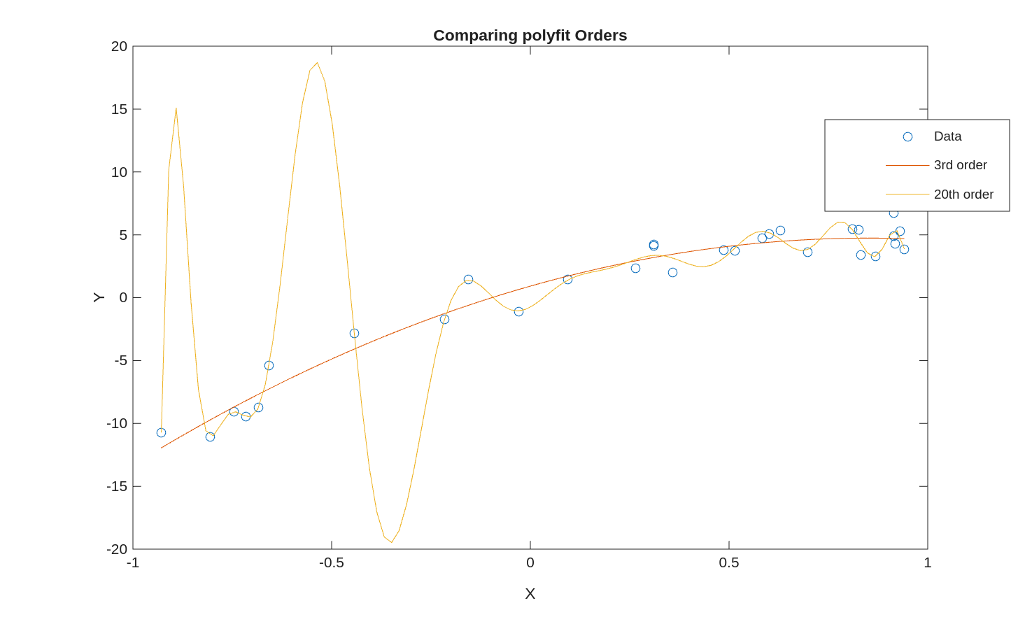
Sometimes we are in a situation where we have gathered data and we want to find a polynomial approximation that goes through that data. One example would be parameter estimation - where we run an experiment and gather data that is the output of a polynomial but the quantites we are actually interested in are the underlying coefficients. Another example is where generating data points is very expensive and time consuming, like a program that takes days to run, so you could run that program at specific points then approximate the program’s output with a polynomial that fits thost points.
The polyfit function in MATLAB finds the polynomial-of-best-fit for a set of points.
The syntax is p = polyfit(x, y, n), where n is the order of the polynomial.
For a line-of-best-fit, set n to 1.
Polynomial fitting does require some care and understanding of the underlying data.
Setting n to be a large number can cause over-fitting and become very sensitive to changes in the data.
As an example:
% Noisy data
x = [-0.92858 -0.80492 -0.74603 -0.71623 -0.68477 -0.65763 -0.443 -0.21555 -0.15648 -0.029249 0.093763 0.26472 0.31096 0.31148 0.35747 0.48626 0.51548 0.58441 0.60056 0.62945 0.69826 0.81158 0.82675 0.83147 0.86799 0.91433 0.91501 0.91898 0.92978 0.94119];
y = [-10.7164 -11.073 -9.0585 -9.4775 -8.7553 -5.414 -2.8329 -1.6983 1.4228 -1.1005 1.4619 2.3122 4.0963 4.2178 2.014 3.7819 3.7146 4.7525 5.0552 5.3227 3.5928 5.4527 5.3819 3.4203 3.3068 4.8925 6.7389 4.2669 5.2606 3.8293];
plot(x, y, 'o')
hold on

x_plt = linspace(min(x), max(x), 101); % higher resolution than x

% Quadratic fit
p_quad = polyfit(x, y, 2);
plot(x_plt, polyval(p_quad, x_plt))

% 20th order fit
p_20th = polyfit(x, y, 20);
plot(x_plt, polyval(p_20th, x_plt));

% Format plot
hold off
xlabel('X')
ylabel('Y')
legend('Data', '3rd order', '20th order')
title('Comparing polyfit Orders')
The MATLAB Help Center has documentation on polyfit.
Reading Questions
- How do you evaluate a polynomial with coefficients in the array
pat specific values ofx? - Does the order of coefficients in
pmatter? If so, how should they be ordered? - What should the array
pbe for the polynomial $9 x - x^5$? - What additional step must be done in order to add or subtract polynomials?
- How do you get the roots of a polynomial from its coefficients?
- How do you get the coefficients of a polynomial from its roots?
- What are the outputs of the
deconvfunction? - How would you raise a polynomial to the power 2? What about the power 5?
- How can you find the line-of-best fit?
- What should you consider when deciding the order of the polynomial-of-best-fit?