Complex Numbers
Complex numbers extend the real number system by introducing an imaginary component. This component multiplies the imaginary number $i=\sqrt{-1}$, which is sometimes called $j$. MATLAB natively supports complex numbers, and has several features that facilitate working with them. Though complex numbers do not “exist” in the real world, they are tremendously useful in engineering design and analysis. They make it easier to understand circuits with alternating current, control systems, and vibrations.
\[z = a + b i\]The complex number $z$ has real component $a$ and imaginary component $b$. The MATLAB Help Center has a guide on Complex Numbers
Creating Complex Numbers
MATLAB has two methods for creating complex numbers.
You can either type it the way it is written,
or construct it with the complex function.
For example:
z1 = 3 + 4i
z2 = -1.2 - 2j
z3 = complex(8, -8)
z1 =

   3.0000 + 4.0000i


z2 =

  -1.2000 - 2.0000i


z3 =

   8.0000 - 8.0000i
You can also create arrays of complex numbers. For instance:
z = [1+2i, 3-4i; -5i, 6];
Once a complex number has been defined, you can access its
real and imaginary components using the real and imag functions.
Both i and j are available for the imaginary number.
Sometimes i is used to index into an array, like the $i$-th term,
which would overwrite the built-in definition of $\sqrt{-1}$.
Best practice is to avoid short variable names,
so a(idx) is preferred over a(i) because its clearer
what the variable is used for and avoids overwriting the imaginary number.
The MATLAB Help Center has documentation on complex, real, and imag.
Basic Arithmetic
Just like real numbers, we can do basic arithmetic with complex numbers. This includes addition, subtraction, multiplication, division, and exponentiation. Using the complex numbers from the previous section:
complex_examples;  % loads z1,z2,z3 from previous section

% Addition and Subtraction
z_sum = z1 + z2
z_diff = z1 - z2

% Multiplication
z_prod = z1 * z2

% Division
z_quot = z1 / z2

% Exponentiation
z_pow = z1 ^ 2
z_sum =

   1.8000 + 2.0000i


z_diff =

   4.2000 + 6.0000i


z_prod =

   4.4000 -10.8000i


z_quot =

  -2.1324 + 0.2206i


z_pow =

  -7.0000 +24.0000i
Addition and subtraction are done separately on the real and imaginary components of the complex numbers. The product follows the FOIL rule of first-outside-inside-last. Internal to MATLAB, the quotient is found by taking the complex conjugate of the denominator. This inverts the denominator, so essentially:
\[\frac{z_1}{z_2} \RightArrow z_1 z_2^{-1} \RightArrow z_1 \bar{z_2} \frac{1}{|z_2|^2}\]Finally, exponentiation is repeated multiplication.
Polar Form
Complex numbers can be expressed in polar coordinates (radius and angle) in addition to the Cartesian (real and imaginary) coordinates. This makes use of the identity:
\[r e^{i\theta} = r \cos(\theta) + r \sin(\theta) i\]To access the complex magnitude $r$, use the abs function.
The angle can be accessed using the angle function.
The result from angle is always expressed in radians.
For example:
complex_examples;  % loads z1,z2,z3 from previous section

% Magnitude
z1_norm = abs(z1)
z2_norm = abs(z2)
z3_norm = abs(z3)

% Angle
z1_ang = angle(z1)
z2_ang = angle(z2)
z3_ang = angle(z3)

z3_ang_deg = 180*z3_ang/pi
z1_norm =

     5


z2_norm =

    2.3324


z3_norm =

   11.3137


z1_ang =

    0.9273


z2_ang =

   -2.1112


z3_ang =

   -0.7854


z3_ang_deg =

   -45
The MATLAB Help Center has documentation on abs and angle.
Conjugation and Symmetry
The complex conjugate of a number $z = a + bi $ is defined as:
\[\bar{z} = a - bi\]In MATLAB, you compute the conjugate using the conj function:
zc = conj(z);
Conjugation reflects points across the real axis in the complex plane. We often see conjugate pairs as the complex roots to the quadratic formula, like $r = a \pm b i$. For any general polynomial, if it has a complex root then the conjugate is also a root. This symmetry across the real axis underlies many algorithms in signal processing and control systems. It guarantees that real-world responses remain real, cancelling out imaginary components.
Example: AC Circuit Impedance
Question
Consider a circuit with a resistor, inductor, and capacitor (RLC) all in series. Current flowing through this circuit will experience an effective impedance, which is like resistance but depends on the frequency of the alternating current.
The circuit has the following properties:
- Resistance, $R =$ 100 $\Omega$
- Inductance, $L =$ 0.2 $H$
- Capacitance, $C =$ 10 $\mu F$
The impedance of the RLC circuit depends on both the properties above and the frequency, $\omega$, of the alternating current:
\[Z = R + j\omega L - \frac{j}{\omega C}\]First, find the inductance of the circuit when $\omega$ = 1,000 rad/s, as well as the magnitude and phase angle (in degrees).
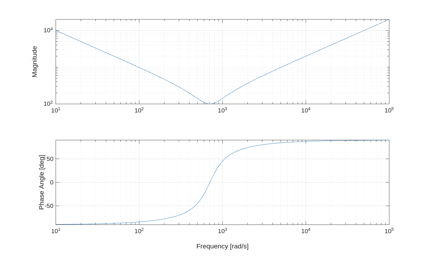
Second, create a plot with two subplots for the magnitude and phase, with the magnitude plot on top and the phase plot beneath it. The x-axis of these plots should be frequency, ranging from 10 rad/s to 10,000 rad/s, and in log scale. The y-axis should be magnitude and phase, respectively. The y-axis of the magnitude plot should be log scale, while the y-axis of the phase plot should be linear scale with units of degrees. Turn the grid lines on in both subplots.
Solution
%% Givens

R = 100;
L = 0.2;
C = 10e-6; % uF means 10^-6 Farad

%% Part 1
omega = 1000;

Z = R + j*omega*L - j/(omega*C)

mag = abs(Z)
phase = rad2deg(angle(Z))

%% Part 2

% same as Part 1 but for range of omega
omega = 10.^linspace(1, 5, 500);

Z = R + j*omega*L - j./(omega*C);

mag = abs(Z);
phase = rad2deg(angle(Z));

% create subplots
tiledlayout(2,1);
ax1 = nexttile;
loglog(omega, mag)
ylabel('Magnitude')
grid on

ax2 = nexttile;
semilogx(omega, phase)
xlabel('Frequency [rad/s]')
ylabel('Phase Angle [deg]')
ylim([-90, 90]) % cleaner result than the default
grid on
To find the solution to the first part, we list the givens and calculate $Z$ according to the equation above.
The magnitude is found with the abs function and the angle with the angle function.
To convert the angle to degrees, I used the rad2deg function.
You can also multiply by pi/180.
These are the results:
Z =

   1.0000e+02 + 1.0000e+02i


mag =

  141.4214


phase =

    45
The second part is the same as the first, except now $\omega$ is a range from 1 to 100 rad/s.
I chose make omega to be linear in the powers of 10 so there would be better spacing between grid points.
The specific values between 1 and 100 rad/s were not specified, so anything that makes the plots look smooth is fine.
This is the plot:
Reading Questions
- In a complex number, what is the definition of $i$ and $j$?
- What is the complex conjugate of the number $5 + 3j$ ?
- How do you convert a magnitude and phase angle into a complex number?
- How do you find the magnitude and phase angle of a complex number?
- Why are complex numbers used in engineering if they don’t “exist” in the real world?