History of Computing

Introduction

Computation, at its core, involves the processing of data and execution of instructions to solve problems. From ancient mechanical devices to modern supercomputers, the field of computation has revolutionized how engineers, scientists, and mathematicians address complex challenges.

Modern engineers often perform computations on personal computers, when it would be more time-intensive or error-prone to do by hand. Some computations, such as simulating turbulent flows, may grow beyond the limits of a personal computer and require the use of computer clusters. Others may be performed remotely, such as a rocket steering itself through launch. This page highlights the most important computing advances through history, from the abacus to the modern computer.

Early Beginnings: Mechanical Computation

The foundations of computation began with mechanical devices designed to aid calculations. Ancient cultures like the Babylonians and Egyptians used tools such as the abacus for arithmetic tasks. Farmers, for example, would use the abacus to track how many heads of cattle they owned. The Inca used a system of knots to both add large numbers and record the individual terms of the sum.

A significant leap occurred in 1614, when John Napier invented logarithms. In the early 1620s, William Oughtred invented the slide rule and fundamentally changed the way we performed multiplication, division, exponentiation, trigonometry, and solving the quadratic formula. Use of the slide rule only declined in the 1970s when they were replaced by handheld calculators. To learn more about multiplying and dividing with a slide rule, visit Basic Slide Rule Use.

Glenn L. Martin Hall, on the University of Maryland College Park campus, was designed to look like a slide rule from above. (aerial view)

It is worth noting at this point that the abacus adds and subtracts in discrete steps, while the slide rule is continuous. For example, an abacus cannot add an irrational number (e.g. \(\pi\)) without rounding first. Slide rules can be used without rounding, limited instead by the user’s ability to line up the rules and cursor. Though this may seem like an advantage for continuous computing machines, discrete machines would overtake them as technology advanced. Finer resolution, analogous to having many rows on an abacus for the tenths, hundredths, thousandths, and so on, would make round-off error nearly imperceptible.

Traditional suanpan (Chinese abacus) illustrating the use of suspended beads.

Diagram showing the use of a slide rule.

The Age of Machines: 17th to 19th Century

While the slide rule accelerated a long list of mathematical operations, addition and subtraction were not on that list. Decades later in 1642, Blaise Pascal invented the Pascaline: a mechanical calculator capable of addition and subtraction. It used a series of interlocking gears and dials, where each dial represented a digit. Turning the dials would rotate the gears, calculating sums and differences automatically.

Gottfried Wilhelm Leibniz improved on the Pascaline in 1673 with the invention of the Leibniz wheel. The wheel was a gear where the teeth had different widths, so adding a specific number was a matter of sliding the wheel to set how many teeth engaged an axle. All four fundamental arithmetic operations could be performed with a single Leibniz step reckoner, a machine with a Leibniz wheel representing each of the tens places. The stepped reckoner would remain the primary arithmetic machine in use for the next 150 years.

The Montgolfier brothers began ballooning in 1783. Their flights were the start of human aviation, notably including a flight over Paris. It is unlikely they used arithmetic machines, however, as their work was primarily experimental.

Pascaline replica at the National Museum of Science and Technology (Sweden).

Photograph of a Leibniz stepped reckoner discovered in 1879.

The Industrial Revolution enabled mass production of nearly everything, including textiles and arithmetic machines. In 1804, Joseph Marie Jacquard invented a programmable loom that could weave a wide variety of complex patterns, with each pattern punched into a sequence of cards. This improvement in automation, along with several other innovations, lead to significant job losses for skilled textile workers, ignited conflicts across England, and highlighted the social impact of automating people’s jobs. In 1820, Charles Xavier Thomas used the same operating principles as the step reckoner, improving on it with a design that could be mass produced. His design would not reach the market until 1851, in part due to a shift in the British government’s focus to the difference engine invented by Charles Babbage.

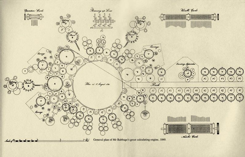
The Babbage difference engine was notable for its ability to evaluate polynomials. Previously, transcendental functions like sine and cosine were evaluated by looking up values in tables. The publishers for these tables calculated and recorded values by hand - for a limited number of angles. Babbage wanted to eliminate all sources of human error from tabulating these values and devised a machine that could calculate the next row in a table based on the previous row and some intermediate values. It was known for a century by this point that these functions could be approximated by a polynomial series, such as

\[\sin(x) \approx x - \frac{x^3}{3!} + \frac{x^5}{5!} + ...\]

Babbage’s difference engine could be set with the coefficients of a polynomial, then evaluated for a specific input value. Charles Babbage spent 19 years developing and building the difference engine, abandoning the project to create a programmable machine like the Jacquard looms - an engine capable of performing any sequence of calculations. He set to work on the mechanical design of an analytical engine, while Ada Lovelace wrote instructions for the machine, making her the first computer programmer.

Example: Finite Difference Table

Question

Compute the first 5 entries in a finite difference table for the polynomial $f(x) = x-1000 x^5$, starting from $x=0$ and using a step size of $\Delta x = 0.01$. Compare the final value of $f(x)$ in the table with $sin(x)$ computed by calculator and find the percent error. Use the following pre-computed differences:

$x$	$f(x)$	$\Delta f$	$\Delta_2 f$	$\Delta_3 f$	$\Delta_4 f$	$\Delta_5 f$
0	0	0.01	-3e-6	-1.5e5	-2.4e-5	-1.2e-5

Solution

We start by populating the first row with the pre-computed differences. In the next row, $\Delta_5$ remains constant, while $\Delta_4^{(new)}=\Delta_4^{(old)} + \Delta_5^{(old)}$. The same applies for $\Delta_3$ and so on for the entire row. This procedure is repeated for each row until we have 5 new rows. Values below are given with 3 significant digits, but calculated with machine precision.

$x$	$f(x)$	$\Delta f$	$\Delta_2 f$	$\Delta_3 f$	$\Delta_4 f$	$\Delta_5 f$
0	0	0.01	-3.00e-6	-1.50e-5	-2.40e-5	-1.20e-5
0.01	1.00e-2	0.01	-1.80e-5	-3.90e-5	-3.60e-5	-1.20e-5
0.02	2.00e-2	9.98e-3	-5.70e-5	-7.50e-5	-4.80e-5	-1.20e-5
0.03	3.00e-2	9.92e-3	-1.32e-4	-1.23e-4	-6.00e-5	-1.20e-5
0.04	3.99e-2	9.79e-3	-2.55e-4	-1.83e-4	-7.20e-5	-1.20e-5
0.05	4.97e-2	9.53e-3	-4.38e-4	-2.55e-4	-8.40e-5	-1.20e-5

The final value in the table is 0.0496875. Computing the polynomial directly, using Microsoft Excel, yields 0.0496875. There is 0% error between the method of finite differences and the direct calculation.

The significant improvement with the analytical engine was that the output of one calculation could be passed as input to another calculation. The specific operations in each calculation step would be defined by the user with a punch card system, inspired by the Jacquard looms. Though the analytical engine would never be built, the concepts of listing operations and storing values in memory became fundamental to modern computing.

During this time, Henri Giffard invented a steam-powered dirigible and Otto Lilienthal developed winged gliders. Their work was primarily experimental, supplemented by calculations made with slide rules and graphical techniques. The Wright brothers similarly relied on experimental methods, though they also performed calculations with slide rules and charts.

Jacquard loom in Norrkoping City Museum (Sweden).

Arithmometer from the late 1890s.

Babbage difference engine No. 1 in Science Museum (London).

Babbage analytical engine, with the "CPU" on the left and "memory" on the right. Science Museum (London).

The video below demonstrates the working of Babbage’s Difference Engine No. 2, an improved design that was realized later in 1991.

The Rise of Electronic Computing: 20th Century

The early 20th century marked a pivotal shift from mechanical computation to electronic systems. As technological capabilities grew, engineers sought faster, more reliable ways to process information.

Theoretical Foundations

In 1936, Alan Turing introduced the concept of the Turing Machine. This abstract mathematical model defined the principles of computation. His work laid the theoretical groundwork for modern computer science. It demonstrated that any algorithmic process could be represented with a set of logical steps.

A Turing Machine operates like a basic mechanical computer that follows a set of rules to manipulate symbols on an infinite tape. Imagine the tape as a long row of boxes, each containing a single character. A read/write head moves along the tape, examining one box at a time and following predefined instructions. At each step, the machine can:

• Read the symbol in the current box.
• Write a new symbol in the box, replacing the old one.
• Move left or right along the tape to examine the next box.
• Change its internal state, which helps track progress in solving a problem.

Although this machine is simple, it is capable of performing any step-by-step computational task. Modern computers work similarly—they process information by following sequences of instructions stored in memory. Just as a Turing Machine can execute a series of logical steps, today’s processors execute programs by manipulating numbers and symbols according to rules set by a programmer. The fundamental ideas behind the Turing Machine—storing, reading, and modifying data sequentially—are key to understanding how software operates on hardware.

This simple yet powerful model established the theoretical limits of computation. It led to the Church-Turing Thesis, which states that any function computable by an algorithm can be computed by a Turing Machine. This principle underpins modern programming languages and computer architecture. Turing’s work also influenced the development of stored-program computers, where instructions and data are treated similarly.
This concept became the basis for modern digital computers.

Although Turing did not build a physical Turing Machine, his ideas directly influenced real-world computers. During World War II, he worked at Bletchley Park, where he helped design the Bombe, an electromechanical device used to break German Enigma codes. Later, his work contributed to the development of early computers like the ACE (Automatic Computing Engine).

During this time, the Germans developed the V2 rocket, the first long-range guided ballistic missile. It had an onboard analog computing device that measured voltages from gyroscopes and commanded a system of exhaust vanes and rudders, which stabilized the vehicle during flight. This system was more of a signal processor than a computer, however, and a lack of course corrections made them unlikely to reach their target.

Example: Turing Machine

Question

Create the list of steps for a Turing machine that adds 1 to a 4-bit unsigned integer. For example, if the tape holds the binary for 7, 0111, the end result of the steps should be the binary for 8, 1000.

For more information about integers in binary, visit Binary.

Solution

The machine starts at the rightmost digit of the binary number. It follows these rules:

1. If the digit is 0, change it to 1 and halt.
2. If the digit is 1, change it to 0 and move left.
3. Repeat step 2 until a 0 is found or a new digit is added to the tape.

Processing steps:

Step	Tape Content	Read Digit	Action	Updated Tape	Move Direction
1	0111	1	Change to 0	0110	Left
2	0110	1	Change to 0	0100	Left
3	0100	1	Change to 0	0000	Left
4	0000	0	Change to 1	1000	Halt

The final tape content is 1000, the binary representation for 8.

Pioneering Electronic Machines

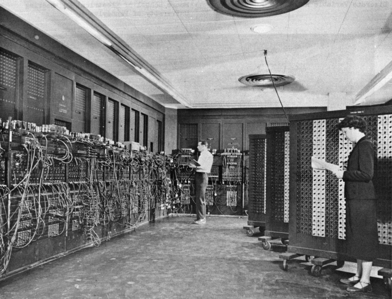
The first practical application of electronic computing emerged in the 1940s with the development of ENIAC (Electronic Numerical Integrator and Computer). Completed in 1945, ENIAC was the first general-purpose electronic computer, meaning it could be programmed to perform different types of calculations instead of being built for a single task. Unlike earlier machines that relied on mechanical components, ENIAC used vacuum tubes—small electronic switches—to process information much faster. This allowed it to perform thousands of calculations per second, a groundbreaking achievement at the time.

ENIAC was primarily designed for military applications, particularly artillery trajectory calculations, which required complex mathematical computations. Its ability to automate these calculations was a significant advantage, as it drastically reduced the time needed to produce firing tables for weapons. While massive—occupying an entire room—it demonstrated the potential of electronic computers in scientific and engineering fields.

As computing technology advanced, companies began developing commercial machines for broader applications. In 1953, IBM introduced the Model 650, one of the earliest computers designed specifically for businesses and universities. Unlike previous systems that relied on vacuum tubes, the Model 650 incorporated magnetic drum memory, a precursor to modern storage devices. This provided a more efficient way to store and retrieve data, making computing more accessible to research institutions and engineers who needed powerful tools for data analysis.

These early machines laid the foundation for the rapid evolution of computing in the decades that followed. They proved that electronic computers could handle complex tasks efficiently, leading to innovations in fields ranging from business and engineering to scientific research. Today’s computers are vastly more powerful, but they owe their existence to these pioneering machines that demonstrated the incredible potential of electronic computation.

Before electronic, programmable computers were widely available, aerospace engineers used a variety of purpose-built analog computing devices. The governing equations for fluid flow, for example, could be approximated with an electrical circuits. The voltage difference between two points could be measured with a voltmeter, then converted into a pressure difference in the flowfield. There was also a water-based computer, where the water level in various reservoirs stored values in the calculation.

ENIAC at Aberdeen Proving Ground, Maryland. Glen Beck (background) and Betty Snyder (foreground) program the ENIAC in building 328 at the Ballistic Research Laboratory.

Computational Power in Engineering: Late 20th Century

The late 20th century witnessed rapid advancements in computational hardware and software. These advancements transformed engineering fields.

The Rise of Personal Computing

The introduction of personal computers in the 1980s revolutionized computation. It made powerful tools accessible to engineers worldwide. Previously, large mainframes dominated the industry. Smaller computers provided flexibility and efficiency.

Key software innovations emerged during this period. One of these was MATLAB (introduced in 1984). It allowed engineers to perform numerical computations, analyze data, and create simulations. MATLAB quickly became a staple in scientific and engineering research. Its ease of use and robust mathematical capabilities made it invaluable.

Computer-Aided Design (CAD) tools also gained prominence. They enabled engineers to develop precise digital models of mechanical components, buildings, and complex systems. This shift significantly improved design accuracy and efficiency.

Supercomputing and Parallel Processing

By the 1990s, supercomputers played a crucial role in solving large-scale engineering problems. Parallel computing became instrumental in fields such as:

• Finite Element Analysis: Modeling stress distributions in materials.
• Fluid Dynamics Simulations: Predicting airflow around aircraft and spacecraft.
• Weather and Climate Modeling: Analyzing large-scale atmospheric patterns.

These advancements paved the way for increasingly sophisticated engineering applications.

The Modern Era: 21st Century and Beyond

Modern computation continues to evolve rapidly. It enables engineers to tackle increasingly complex challenges.

Artificial Intelligence and Machine Learning

The integration of AI and Machine Learning has transformed engineering workflows. Predictive modeling, automated data analysis, and optimization algorithms assist in designing efficient aircraft. They also help manage mechanical systems and advance robotics.

Cloud Computing and Distributed Processing

With the rise of cloud computing, engineers can now perform complex simulations remotely. They can collaborate across different locations without requiring dedicated high-performance hardware on-site. This innovation has improved accessibility and efficiency in research and industry.

Quantum Computing: The Next Frontier

Emerging quantum computing technologies offer revolutionary possibilities for engineering computation. Unlike classical computers that process information as binary bits (0s and 1s), quantum computers leverage qubits. Qubits exist in multiple states simultaneously. This approach could dramatically accelerate calculations for fields like:

• Aerodynamic modeling: Simulating turbulence at unprecedented resolution.
• Structural engineering: Optimizing materials for extreme conditions.
• Cryptography: Enhancing security in aerospace communications.

Summary

The history of computing is a story of continuous innovation, shaping the way humans process information, solve complex problems, and interact with technology. Early mechanical devices laid the foundation of representing numbers with the state of the machine, and programmable machines ushered the dawn of computer science. Vacuum tubes, and later transistors, reduced the physical size of the devices storing numbers and accelerated the rate of computation. Though modern hand-held devices contain more computing power than the early room-sized computers, we continue to use large-scale computer clusters and supercomputers for increasingly sophisticated calculations. Today, computing is woven into every aspect of life, driving scientific discoveries, business operations, and global communication.

Reading Questions

1. Which arithmetic operations (add, subtract, multiply, divide, exponentiation, logarithm) are done with the abacus?

2. Which arithmetic operations are done with a slide rule?

3. Which part of the Jacquard looms was adapted for computing machines?

4. How did Babbage’s Analytical Engine improve on the Difference Engine?

5. What was Ada Lovelace’s role with the Analytical Engine?

6. How did the Turing Machine impact computer design?

7. Why is the ENIAC considered a revolutionary machine?

8. How did the widespread adoption of personal computers, beginning in the 1980s, changed the practice of engineering?